The workflow that keeps a backtest honest
A backtest returns one number, and one number is exactly what an overfitted strategy is best at producing. The work that follows is what separates an edge from a coincidence: draw the map, validate on data you did not fit, bound the luck, check that nothing read the future. Each of those is one call here, and the figures below are one strategy going through all of them, on real BTC-USDT perp bars.
The whole fold loop runs natively, so validation costs about what the sweep inside it costs.
Four questions one backtest cannot answer
They are not stages you can skip in a hurry, they are four different ways of being wrong. A strategy can pass any three and fail the fourth.
Is this a region or a point?
sweepA single Sharpe says nothing about what happens one parameter step away. A 2D sweep draws the surface the number sits on, and a stability score puts a figure on how much it moves when a parameter does. A peak with a cliff on either side is not a strategy, it is a coincidence with good manners.
Does it survive data it has not seen?
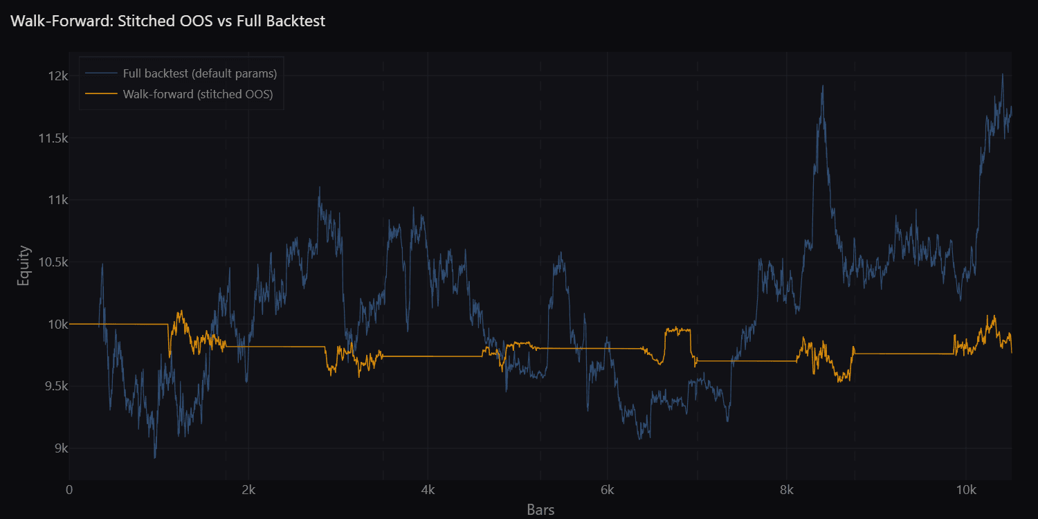
walk-forwardParameters chosen on one window, measured on the next, fold after fold, so the number you read was never optimised for. The stitched out-of-sample curve is the honest one, and comparing it to the full-sample backtest tells you what the fitting bought.
How much of this was luck?
monte carloResample the returns to bound the tail and the probability of ruin. Shuffle their order to see how much of the equity curve was the sequence rather than the edge. A strategy whose result depends on one lucky ordering is telling you something.
Did the strategy see the future?
diagnosticsLook-ahead does not announce itself: it just produces a beautiful equity curve. The detector cross-examines your strategy on your own data and fails it if the result depended on information that was not available at the time, naming the signal responsible rather than leaving you to guess.
Draw the map, then find where you are standing on it
Picking the best cell of a grid is how strategies get overfitted. The useful reading is the neighbourhood: a broad plateau survives a parameter being slightly wrong, and a lone spike does not survive next month.
import manifoldbt as mbt

# The map: one metric over two parameters, as a single native call.
# This is the figure beside it: 500 x 500 = 250,000 backtests of an EMA
# crossover on BTC-USDT perp hourly bars, 2021-2025, in 19.7 s on the CPU.
heat = mbt.run_sweep_2d(
    strategy,
    {
        "x_param": "fast", "x_values": list(range(2, 502)),
        "y_param": "slow", "y_values": list(range(10, 1010, 2)),
        "metric": "sharpe",
    },
    config, store,
)
mbt.plot.heatmap_2d(heat, annotate=False)

# The score: how much that metric moves when one parameter moves.
stab = mbt.run_stability(
    strategy,
    {"param_name": "slow", "values": list(range(50, 1010, 25)), "metric": "sharpe"},
    config, store,
)
stab["stability_score"], stab["mean_metric"], stab["std_metric"]
# -> 0.34, 0.41, 0.27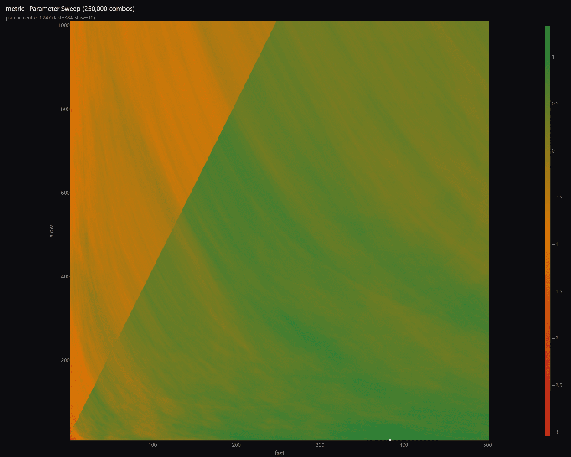
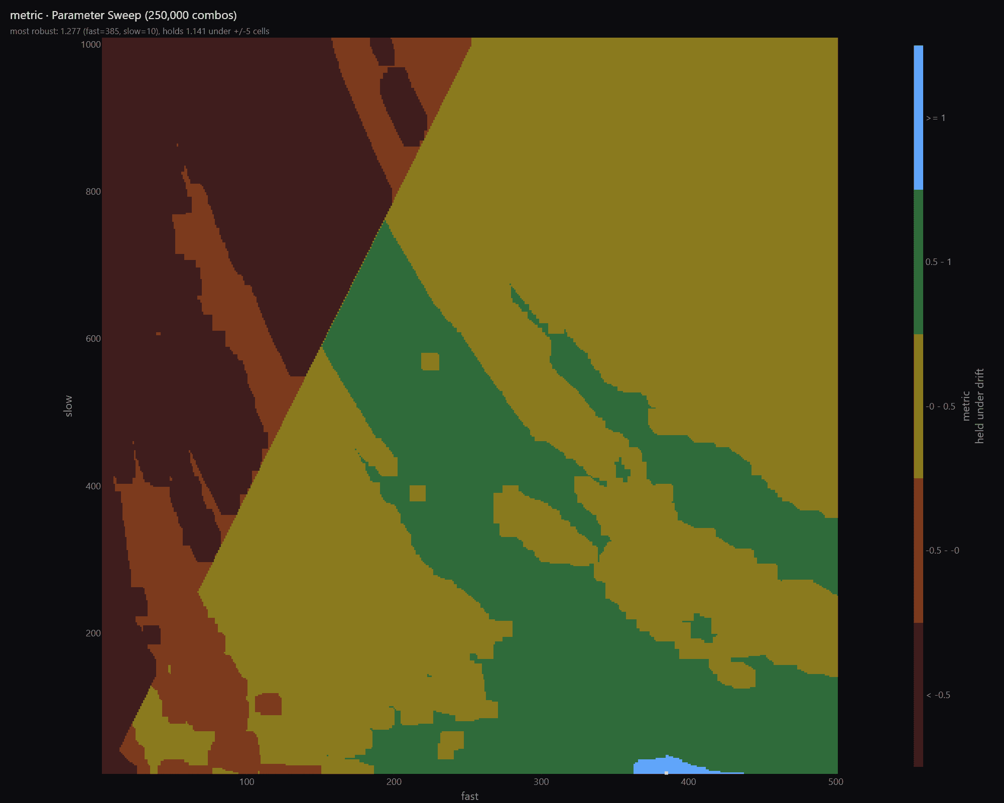
Scanning one parameter at a time puts a number on the same idea. Sweeping the slow period from 50 to 1,000 gives a mean Sharpe of 0.41 with a standard deviation of 0.27, and a stability score of 0.34: the result moves almost as much as it is worth. That is the first warning, and the next section is where it gets confirmed. Drawing the map is cheap enough to be a habit rather than an event, a quarter of a million backtests in twenty seconds here and 5,041 in 0.41 s on a hundred thousand bars, measured on the engine page. When the map itself gets big enough to hurt, that is what the GPU path is for.
Walk-forward: optimise on one window, measure on the next
Four geometries cut the folds: anchored keeps every past bar, pardo slides a fixed window, blocked uses disjoint blocks, custom leaves both axes free. Whichever you pick, the parameters for a fold are chosen without the data they are then judged on, which is the only way an in-sample optimiser can produce a number worth reading.
wf = mbt.run_walk_forward(
    strategy,
    {
        "geometry": "blocked",      # or "anchored": keep every past bar
        "n_splits": 6,
        "train_ratio": 0.7,
        "optimize_metric": "sharpe",
        "param_grid": {
            "fast": [10, 20, 40, 80, 120, 200, 300],
            "slow": [50, 100, 200, 400, 600, 800],
        },
    },
    config, store,
)

wf["best_params_per_fold"]   # what the optimiser picked, fold by fold
mbt.plot.walk_forward(wf, mode="stitched", full_result=result)
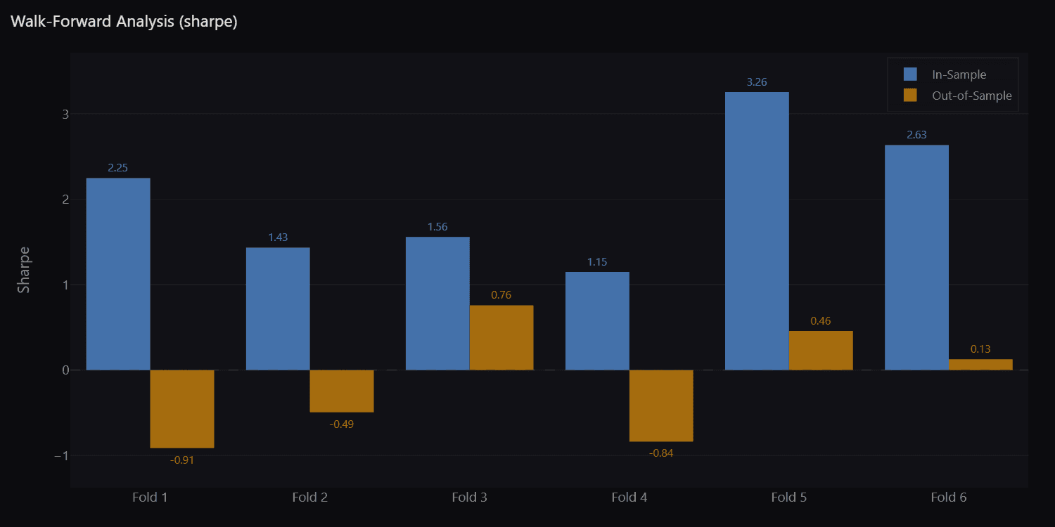
The first thing to read is the gap. Every fold optimises to between 1.15 and 3.26 in sample, and the window immediately after gives it back: -0.91, -0.49, +0.76, -0.84, +0.46, +0.13. Half the folds end negative and none of them keeps a third of what it was fitted to. That is not tuning, that is fitting.
The second is what the optimiser chose. Fast and slow go 20/50, then 10/800, then 300/200, then 10/400, jumping the whole width of the grid between consecutive windows. Parameters that unstable are not tracking a regime, they are chasing noise, and the out-of-sample column is the bill.
For the method itself, step by step and with runnable code, the walk-forward guide goes through a full example.
Monte Carlo: two questions, two methods
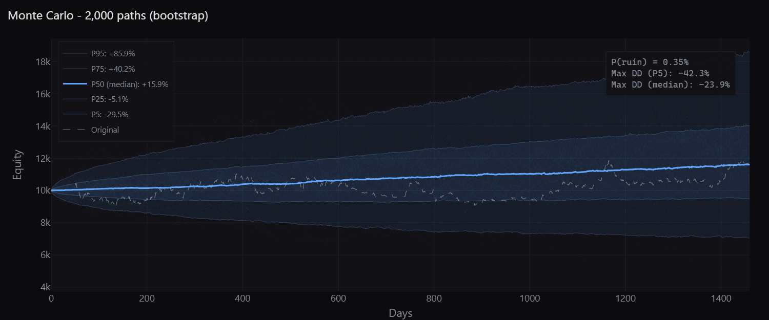
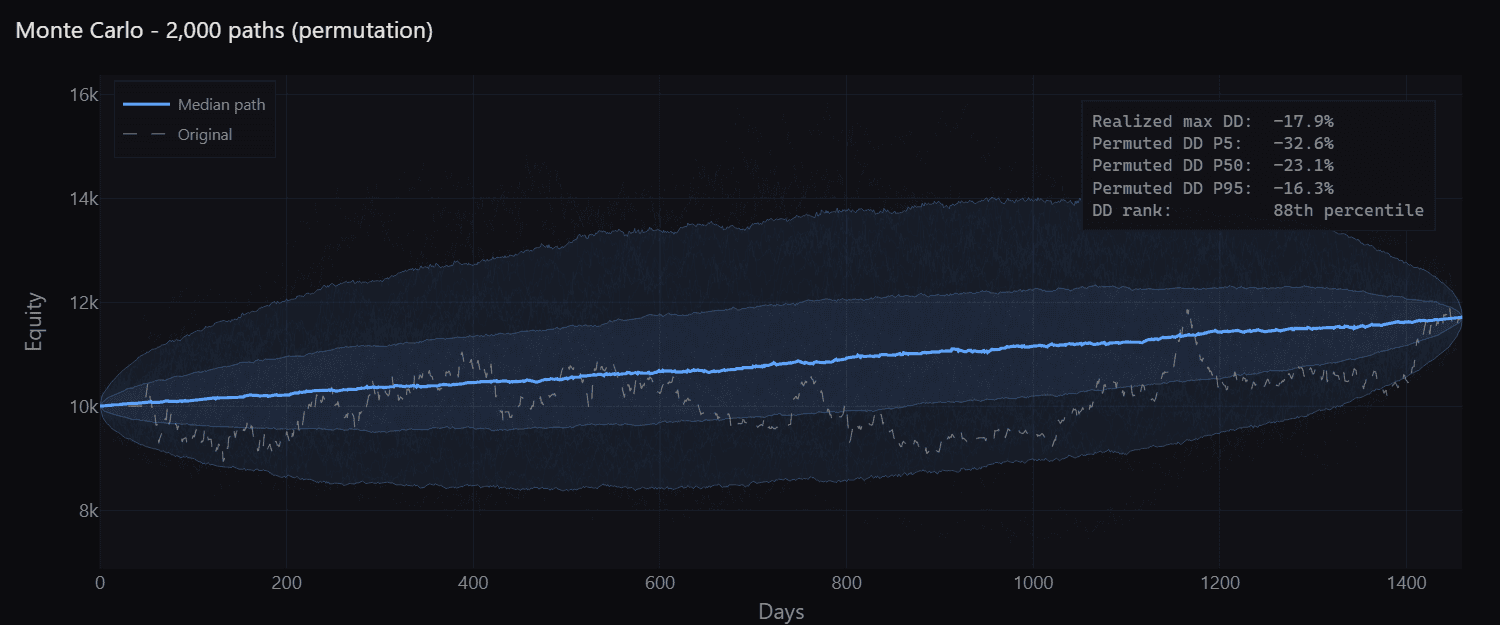
One equity curve is one draw from a distribution you never see. Both methods here rebuild that distribution from the returns you did get, and they answer different questions, so running the wrong one is a quiet way to reassure yourself about nothing. On the run below, the median outcome is +15.9% and the 25th percentile is -5.1%: a quarter of the resampled histories end underwater.
# Bootstrap: resample the returns to bound the tail.
mbt.plot.monte_carlo(result, method="bootstrap", n_simulations=2000, seed=7)

# Permutation: keep the returns, shuffle their order, and see how much
# of the equity curve was the sequence rather than the edge.
mbt.plot.monte_carlo(result, method="permutation", n_simulations=2000, seed=7)
Both are the same call with one argument changed, both are seeded, and both print their own statistics onto the figure, so a chart in a report regenerates exactly and carries its numbers with it. Community runs up to a thousand paths, enough to see the shape; Pro removes the cap, and the tail statistics are the reason to want more of them.
Where this stops working is worth stating plainly: resampling your own returns cannot invent a regime you never traded. It bounds luck within the market you sampled, and nothing beyond it. On a fine-resolution equity curve the path counts that make tail statistics stable get expensive, which is where the GPU bootstrap earns its keep.
The two checks you cannot run by eye
Look-ahead bias does not announce itself. It produces a beautiful equity curve, an excellent Sharpe and no error, and reviewing the code rarely finds it because the mistake usually looks reasonable. The detector goes after it directly, on your own strategy and your own data, and covers both flavours: a statistic computed over the whole sample that leaks backwards, and a signal that quietly uses a bar it should not have seen yet. You get a pass or a fail, with the signal responsible named, and an assertion you can put in CI.
The risk report is the other one: peak utilisation, free margin, leverage against initial capital, and concentration across the universe, over the whole run rather than at the end. A strategy that spends a year at ninety-nine percent utilisation is not the strategy the summary metrics describe.
# Look-ahead: cross-examines the strategy on your own data and raises if
# the result used information that was not available at the time.
mbt.diagnostics.detect_lookahead(strategy, config, store).assert_clean()

# Risk: peak utilisation, free margin, leverage and concentration over the
# whole run, with thresholds you can set.
mbt.diagnostics.risk_check(result).assert_clean()
manifest = result.manifest # strategy, data hashes, engine version, config
# Six months later, on another machine:
again = mbt.replay(manifest, strategy, store)
assert again.metrics == result.metricsA result you can get back
Every run writes a manifest: the strategy definition, hashes of the data it used, the engine version, the whole configuration. Replaying it reproduces the run bit for bit, on another machine and months later.
That is what makes the rest of this workflow worth doing. A validation you cannot reproduce is an anecdote, and a number you cannot regenerate is one you will end up trusting for the wrong reason: because you remember it being good.
FAQ
Explore the rest of the engine
Every capability is documented the same way: what it does, the code that runs it, and the case where it is the wrong tool.
- The Rust Backtesting Engine
A million bars in 22 ms on one core, a grid swept 25x faster than the same backtests one at a time, and where that advantage stops.
- The Expression DSL
Signals declared as composable expressions and evaluated vectorized in Rust: 104 indicators, 38 candlestick patterns, 74 methods, cross-asset references, parameters that sweep.
- Execution Realism
Slippage, fees, funding, borrow, partial fills and decision-to-fill delay, each an independent model rather than one flat cost assumption.
- Multi-Asset Backtesting
Rank a universe on every bar and trade the cross-section: nine perpetuals in one call, one shared account, portfolio-level exposure and fees.
- GPU Acceleration
Parameter sweeps and Monte Carlo on your own NVIDIA GPU, bit-identical to the CPU path, and the measured grid size below which the CPU still wins.
- Options Backtesting
Contracts that expire, cash-settle at intrinsic value, and post margin under a named model: a real multi-leg spread, held to expiry, on live Deribit data.
Find out what your backtest is worth
The map, the folds and the resampling all run on the same engine as the backtest, so validating a strategy costs minutes rather than an afternoon.