What does the engine assume if I configure nothing?

Nothing. Fees are zero, slippage is zero, signal_delay is zero so a signal fills at the close of its own bar, fills are atomic at a single price, and there are no stop or limit orders. That is a deliberately neutral starting point rather than a realistic one: an engine that quietly applied a default cost would make every result depend on an assumption you never made. The corollary is that a first run is optimistic by construction, and the numbers on this page are what that optimism is worth.

Where does funding come from?

From your data. You point the fee config at a funding-rate column in the bars, and the engine applies the rate on the bar it belongs to, so a position pays what it would have paid at the time rather than an average of the period. If the column is not there, funding is simply not modelled, which is visible rather than silent.

Is this an order-book simulation?

No, and it is worth being explicit. The engine models execution at bar resolution: costs, participation limits, intra-bar fill prices, delays and conditional orders. It does not simulate queue position, depth or latency arbitrage. If your edge lives inside the spread or depends on where you sit in the book, this is the wrong tool, and no bar-based backtester is the right one.

Which cost model should I use?

The honest answer is that you should try more than one and look at the spread of outcomes. A flat basis-point cost is a fine first approximation for small size. Volume impact is what you want as soon as your position is a meaningful share of a bar. The useful discipline is not picking the right number, it is checking whether the strategy survives the range of numbers you cannot rule out.

ExecutionCosts

The costs are the strategy

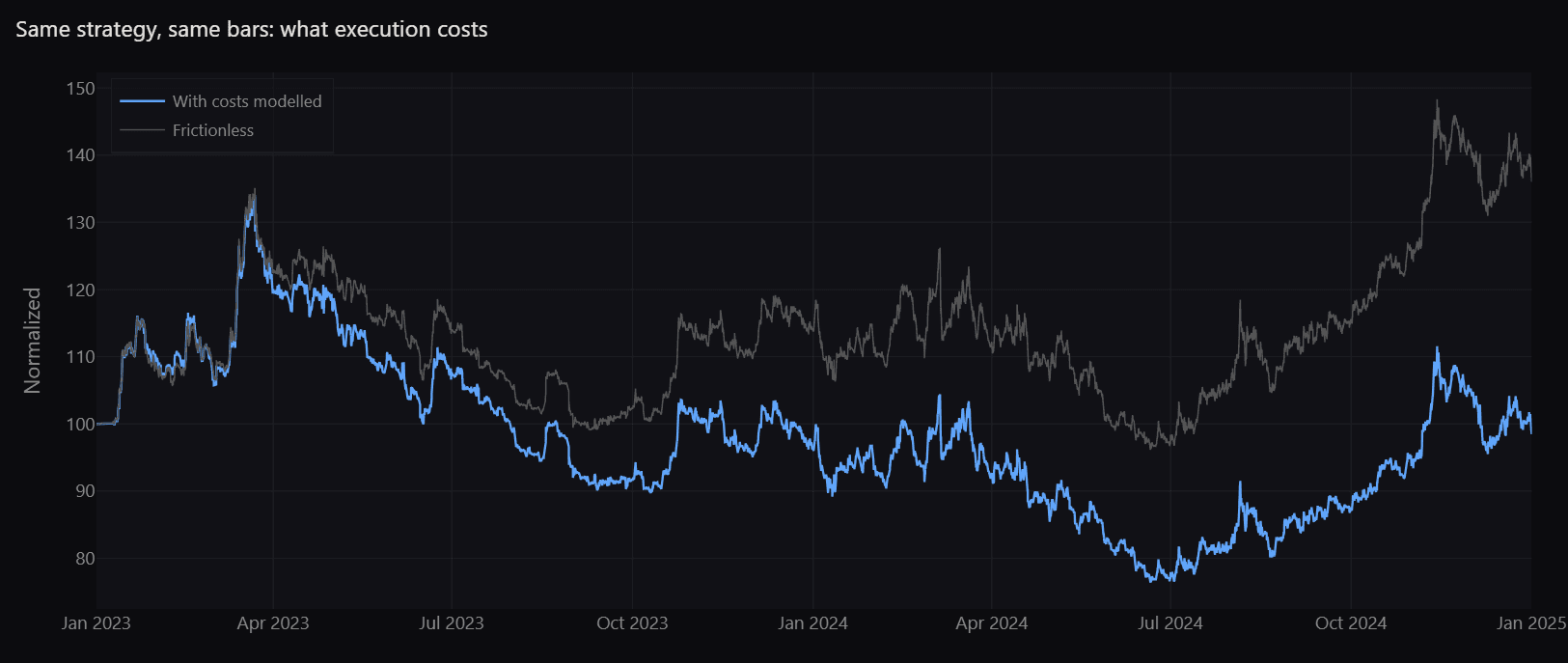
A backtest without execution modelling is a chart of what the price did, not of what you would have earned. Here every cost is its own model, off until you turn it on and configurable when you do: slippage, maker and taker fees, perpetual funding, borrow on shorts, partial fills, and the delay between deciding and filling. The run below lost every point of its return to them.

>>>mbt.ExecutionConfig(signal_delay=1)

The cheapest line of realism you will ever write, and it defaults to zero.

+36% to -1.5%

the same strategy, once the cost models are switched on

0.75 to 0.09

what the Sharpe of that strategy was actually made of

6 models

slippage, fees, funding, borrow, fills and delay, each independent

neutral by default

nothing is assumed for you, which is why you have to look

One strategy, four cost models

Same declaration, same bars, same 427 trades. The only thing that changes between these four runs is what the engine was told about execution, and it is the difference between a strategy worth trading and one that pays its costs to be flat.

Two equity curves from the same strategy over two years: the frictionless run ends near 137 while the run with costs modelled ends near 99 — The same crossover on hourly bars, 2023 and 2024, with and without the cost models. They start together and never reconverge: the grey line ends 37% up, the blue one ends where it started. The gap is not noise, it is the fees, the funding, the impact and the one bar of delay, compounding over 427 round trips.

What was modelled	Sharpe	Return	Max DD
Frictionless	0.75	+36.1%	-28.8%
Flat 5 bp fee, 2 bp slippage	0.14	+0.9%	-42.7%
Same, filled one bar later	0.05	-3.6%	-44.3%
Perp fees, funding, impact, 5% cap	0.09	-1.5%	-43.0%

Read the second row first. Five basis points of fee and two of slippage, the least controversial assumption on the list, take 36 points of return down to one. Nothing exotic happened: the strategy simply trades often enough that costs are the dominant term.

The third row adds one bar of delay between the signal and the fill, and costs another four and a half points. The fourth swaps the flat assumptions for a perpetual-futures setup with real funding, volume-impact slippage and a cap at five percent of each bar’s volume, and lands slightly better than the flat one: at this size, impact is cheaper than a blanket two basis points.

That last detail is the argument for having separate models rather than one number. A flat cost is not conservative, it is just wrong in an unknown direction.

Six models, composed rather than bundled

Each one answers a different question, and each is configured on its own. You can model impact without fees, funding without delay, or all of them at once, and change any of them without touching the strategy.

Slippage

3 models

A fixed number of basis points, a share of the bid-ask spread, or a volume-impact model where the cost is a coefficient times your participation rate raised to an exponent. The third is the one that punishes size, which is the whole reason a strategy that works on paper can fail at scale.

Fees

maker / taker

Separate maker and taker rates in basis points, a minimum fee per trade, and the fill type assumed when the engine cannot know. The default assumption is taker, because it is the conservative one and a backtest that quietly assumes maker fills is a backtest that lies about its edge.

Funding and borrow

carry

Perpetual funding is applied per bar from a funding-rate column in your data, not from an average anyone made up, so a position held through a funding-heavy regime pays what it would have paid. Shorts carry a borrow rate in annualised basis points.

Fills

partial

Cap the share of a bar's volume you are allowed to take and an order that wants more gets filled across bars, which is what actually happens to a large order in a thin market. Choose which price inside the bar the fill lands on: a single point, the typical price, or the OHLC average.

Decision-to-fill delay

latency

signal_delay puts a gap between the bar that produced the signal and the bar that fills it. On fine-grained bars one bar is a realistic decision-to-fill latency; at daily resolution it is a day of drift. It defaults to zero, and on the run below it alone cost four and a half points of return.

Per-venue costs

portfolio

One account can hold instruments that trade in different places, and each venue keeps its own fee schedule and funding column. The costs a portfolio pays are the costs of where each leg actually executes.

import manifoldbt as mbt
from manifoldbt.helpers import Slippage

config = mbt.BacktestConfig(
    # ... universe, time range, bars

    # Each model is independent: change one, leave the rest alone.
    execution=mbt.ExecutionConfig(
        signal_delay=1,                    # decide on this bar, fill on the next
        fill_model={"max_participation_rate": 0.05,   # 5% of the bar's volume
                    "intra_bar_price": "TypicalPrice"},
    ),
    slippage=Slippage.volume_impact(0.1, 1.5),   # coeff * participation ** 1.5
    fees=mbt.FeeConfig(
        maker_fee_bps=2.0, taker_fee_bps=5.0,
        funding_rate_column="funding_rate",       # perpetual funding, per bar
        borrow_rate_annual_bps=300.0,             # cost of carrying a short
        default_fill_type="Taker",                # the conservative assumption
    ),
)

There is no cost preset doing the thinking for you, though there are presets for the venues whose schedules are public, so a perpetual-futures config is one call rather than four numbers you have to look up.

The fill type deserves a moment. It defaults to taker, the expensive side, because the engine cannot know whether your order would have rested or crossed. If your strategy genuinely posts passively, say so explicitly, and be aware that you have just assumed every one of those orders got filled.

For the reasoning behind each model, rather than its API, the deep dive on realistic execution goes through what each one is standing in for.

The defaults are neutral, not realistic

Out of the box there are no fees, no slippage, no delay, and fills are atomic at a single price. That is a decision, not an oversight. A default cost would be an assumption you never made silently deciding whether your strategy works, and the number it produced would look like a result.

It does mean the first run of anything is optimistic, and that the interesting work starts at the second. The one setting worth reaching for immediately is signal_delay: it defaults to zero, which fills at the close of the very bar that produced the signal, and that is only defensible on coarse bars.

Whether the assumptions you did make hold up is a separate question, and the research workflow is where you answer it: sweep the cost parameters like any other and see whether the edge survives the range you cannot rule out.

# Entries and exits as orders, not as instant market fills.
orders = mbt.OrderConfig(
    limit_entry={"price": {"OffsetBps": 10.0},   # rest 10 bps below the close
                 "time_in_force": {"GTB": 5}},   # cancel if unfilled in 5 bars
    stop_loss={"stop_pct": 2.0},
    take_profit={"profit_pct": 5.0},
    trailing_stop={"trail_pct": 3.0, "use_high": True},
)

execution = mbt.ExecutionConfig(signal_delay=1, orders=orders)

Entries and exits can be orders rather than instant fills: a limit resting below the close with a time in force, a breakout that triggers on the way through, a stop, a target, a trailing stop that ratchets on the highs. A stop is filled as a taker with slippage and clamped to the bar; a take-profit fills at its level as a maker. Conditional entries run on the general simulation loop rather than the fast kernel, so a sweep over one is slower than a sweep over a market entry.

Costs follow the instrument, not the backtest

A portfolio that trades in two places pays two fee schedules. Each venue carries its own maker and taker rates, its own funding column and its own minimum, and each instrument is mapped to where it executes.

Leave the mapping empty and everything uses the default schedule, so a single-venue config stays exactly as simple as it was. The multi-asset page covers the rest of what a shared account changes.

# Different instruments, different venues, one account.
fees = mbt.FeeConfig(
    per_venue={
        "venue_a": mbt.VenueFees(maker_fee_bps=2.0, taker_fee_bps=5.0,
                                 funding_rate_column="funding_rate"),
        "venue_b": mbt.VenueFees(maker_fee_bps=10.0, taker_fee_bps=10.0),
    },
    symbol_venue={1: "venue_a", 2: "venue_b"},
)

FAQ

Find out what your edge costs

Every model on this page is in the free version. Turning them on takes a few lines, and it is the cheapest way to find out whether there was anything there.

Read the documentation Why most backtests lie →